Community Opportunity Index

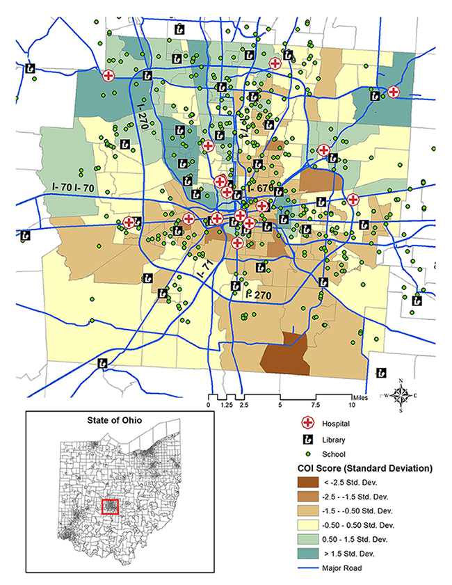
                   Figure: Community opportunity index in Columbus, Ohio

INTRODUCTION

Geographical mapping of community opportunity can help identify social inequity, using a spatially aggregated index comprised of a set of socioeconomic factors. This idea is based on the concept of “neighborhood effects” that where people live influences their socioeconomic outcomes (Acevedo‐Garcia et al., 2004; Jencks and Mayer, 1990). A community opportunity index (COI) can be computed by combining a set of un-weighted standardized neighborhood factors and mapped by using GIS. Wang and Chen (2017) applied this approach to compute a COI for visualizing, identifying, and analyzing the spatial opportunity and deprivation in Columbus, Ohio.

METHOD

In order to create a community opportunity index (COI), physical and socioeconomic data were collected to evaluate the community performance for the neighborhoods in Columbus, Ohio. Census tract data were used as the neighborhood proxies. The following table shows the descriptive statistics of the composite variables in four categories, including economic opportunity, education and child-wellbeing, housing and neighborhood quality, and mobility and accessibility. Data sources include the estimates in 2006-2010 American Community Survey (ACS), the General Transit Feed Specification (GTFS) database, Ohio School Report Cards, the 2010 Census Summary File 1, and Census Transportation Planning Products (CTPP). There are two steps to construct the COI. First, a set of Z-scores are calculated for each tract by standardizing the factors reported in the Table. Secondly, these Z-scores are combined in equal weight to be the COI. Z-Scores for negative factors were multiplied by −1 to create composite scores that represent low-to-high opportunity. A tract with a positive score tends to have a better opportunity, and vice versa.

RESULTS

The spatial distribution of the computed COI, together with main roads, hospitals, schools, and libraries, is illustrated in the Figure below. Several spatial clusters with high COI scores are located in the north, such as Upper Arlington, Worthington, Dublin, and New Albany. In the meantime, vulnerable communities mostly cluster around the city center and in the south. In addition, an ArcGIS shapefile of the COI outcomes can be downloaded using the following link.

Table: Definition and descriptive statistics of community opportunity composite variables

REFERENCES

- Acevedo‐Garcia, D., Osypuk, T.L., Werbel, R.E., Meara, E.R., Cutler, D.M., Berkman, L.F., 2004. Does housing mobility policy improve health? Housing Policy Debate 15, 49-98.
- Jencks, C., Mayer, S.E., 1990. The social consequences of growing up in a poor neighborhood. Inner-city poverty in the United States 111, 186.
- Wang, C-H. and Chen, N.,2017. A geographically weighted regression approach to investigating the spatially varied built-environment effects on community opportunity. Journal of Transport Geography 62, 136-147.
Click on the link below to download the zip file:
COI Shapefile